Measurement of loudspeaker parameters: A pedagogical approach

Download the data file: meas_data.mat
Download the Matlab script file: Loudsepaker_advanced_parameters.m

%% Load the data (from measurements)
load('meas_data.mat');

%% Input Impedance
Z = U./I;

figure;
semilogx(frequencies, abs(Z), 'linewidth', 3);
grid on
xlabel('Frequency [Hz]')
ylabel('|Z_{in}| [\Omega]')
xlim([10, 20e3])
ylim([0, 25]);

Electromagnetic part

$Bl$ estimation

loop through Bl to get the voice-coil impedance $Z_e$ flat

In the Thiele-Small model, the input impedance is
$$Z_{in}(\omega) = R_e + j \omega L_e + Bl \dfrac{V(\omega)}{I(\omega)}$$.
In a more general sense, where the voice-coil impedance is expressed as $Z_e(\omega)$
$$Z_{in}(\omega) = Z_e(\omega) + Bl \dfrac{V(\omega)}{I(\omega)}$$
The voice-coil impedance $Z_e(\omega)$ is then
$$Z_e(\omega) = Z_{in}(\omega) - Bl \dfrac{V(\omega)}{I(\omega)}$$
The voice-coil impedance $Z_e(\omega)$ has no reason to exhibit any kind of resonance at low frequencies. The resonance behavior is due to the mechanical part, in other words due to the term $Bl \dfrac{V(\omega)}{I(\omega)}$. Consequently, we can estimate the $Bl$ value by arbitrarily choosing the estimated value $\overline{Bl}$ that minimizes the resonant behavior of $Z_e(\omega)$, as shown in the following code.

%% Bl estimation
% loop through Bl to get the voice-coil impedance Z_e flat
test_Bl = 0:7;

% real part test
figure;
for Bl = test_Bl
    Zel = Z - Bl*V./I;
    semilogx(frequencies, real(Zel), 'linewidth', 2);
    hold on
end
hold off

legend([repmat('Bl = ',length(test_Bl),1) num2str(test_Bl.') repmat(' Tm',length(test_Bl),1)], 'location','southeast')
grid on
xlabel('Frequency [Hz]')
ylabel('real(Z_e) [\Omega]')
xlim([10, 20e3])
ylim([0, 25]);

% imaginary part test
figure;
for Bl = test_Bl
    Zel = Z - Bl*V./I;
    semilogx(frequencies, imag(Zel), 'linewidth', 2);
    hold on
end
hold off

legend([repmat('Bl = ',length(test_Bl),1) num2str(test_Bl.') repmat(' Tm',length(test_Bl),1)], 'location','southeast');
grid on
xlabel('Frequency [Hz]')
ylabel('imag(Z_e) [\Omega]')
xlim([10, 20e3]);

%% Now we know that Bl should be somwhere beween 4 and 5, so we narow the Bl search
test_Bl = 4.4:0.2:5.4;

% real part test
figure;
for Bl = test_Bl
    Zel = Z - Bl*V./I;
    semilogx(frequencies, real(Zel), 'linewidth', 2);
    hold on
end
hold off

legend([repmat('Bl = ',length(test_Bl),1) num2str(test_Bl.') repmat(' Tm',length(test_Bl),1)], 'location','southeast')
grid on
xlabel('Frequency [Hz]')
ylabel('real(Z_e) [\Omega]')
xlim([10, 1e3])
ylim([4, 8]);

% imaginary part test
figure;
for Bl = test_Bl
    Zel = Z - Bl*V./I;
    semilogx(frequencies, imag(Zel), 'linewidth', 2);
    hold on
end
hold off

legend([repmat('Bl = ',length(test_Bl),1) num2str(test_Bl.') repmat(' Tm',length(test_Bl),1)], 'location','southeast')
grid on
xlabel('Frequency [Hz]')
ylabel('imag(Z_e) [\Omega]')
xlim([10, 1e3]);
ylim([-2, 3]);

%% choose the best Bl
Bl = 4.8;

Voice-coil impedance $Z_e$

%% Voice-coil impedance Ze
Ze = Z - Bl*V./I;

figure
semilogx(frequencies, abs(Ze), 'linewidth', 3)
grid on
xlabel('Frequency [Hz]')
ylabel('|Z_e| [\Omega]')
xlim([10, 20e3])
ylim([0, 25]);

%% real part of Ze (should equal Re)
Re = real(Ze);

figure;
plot(frequencies./1000, Re, 'linewidth', 3)
grid on
xlabel('Frequency [kHz]')
ylabel('apparent R_e [\Omega]')
xlim([0, 20])
ylim([0, 25]);

%% imag part of Ze over omega (should be Le)
omega = 2*pi*frequencies;
Le = imag(Ze)./omega;

figure;
plot(frequencies/1000, 1000*Le, 'linewidth', 3);
grid on
xlabel('Frequency [kHz]')
ylabel('apparent L_e [mH]')
xlim([0, 20])
ylim([0, 1]);

Mechanical part

Mechaical (with acoustical load) impedance $Z_{ma}$

%% Mechanical part

%% Mechancial Impedance Zma
% frequnecy region to 4kHz
idx_cut_modes = find(frequencies > 4000, 1);
freq_axis = frequencies(1:idx_cut_modes);
Zma = Bl*I(1:idx_cut_modes)./V(1:idx_cut_modes);

figure;
semilogx(freq_axis, abs(1./Zma), 'linewidth', 3)
grid on
xlabel('Frequency [Hz]')
ylabel('|Y_{ma}| [mN^{-1} s^{-1}]')
xlim([10, 4e3]);

figure;
semilogx(freq_axis, abs(Zma), 'linewidth', 3)
grid on
xlabel('Frequency [Hz]')
ylabel('|Z_{ma}| [Nsm^{-1}]')
xlim([10, 4e3])
ylim([0, 150])

Mechanical resistance $R_{ma}$

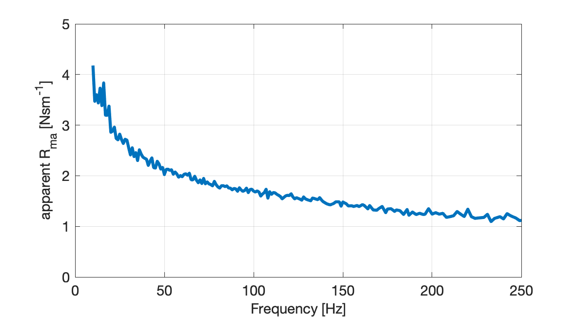
%% Remove the break-up behavior (vibrometer) at frequencies > 250Hz
idx_cut_breakup = find(frequencies > 250, 1);
Zma = Bl*I(1:idx_cut_breakup)./V(1:idx_cut_breakup); % cut all the values of V being over 250Hz
freq_axis_MECH = frequencies(1:idx_cut_breakup);
omega_MECH = 2*pi*freq_axis_MECH;

figure;
plot(freq_axis_MECH, real(Zma), 'linewidth', 3)
grid on
xlabel('Frequency [Hz]')
ylabel('apparent R_{ma} [Nsm^{-1}]')
xlim([0, 250])
ylim([0, 5]);

Mass and Stiffness

%% Mass and Stiffness
test_Mma = 15:20;

figure;
for Mma = test_Mma
    Kma = omega_MECH.^2 * Mma/1000 - omega_MECH.*imag(Zma);
    plot(freq_axis_MECH, Kma/1000, 'linewidth', 2);
    hold on
end
hold off

legend([repmat('Mma = ',length(test_Mma),1) num2str(test_Mma.') repmat(' g',length(test_Mma),1)], 'location', 'best')
grid on
xlabel('Frequency [Hz]')
ylabel('apparent K_{ma} [Nmm^{-1}]')
xlim([0, 250]);

% mass fine
test_Mma= 15.8:0.2:16.6;

figure;
for Mma = test_Mma
    Kma = omega_MECH.^2*Mma/1000 - omega_MECH.*imag(Zma);
    plot(freq_axis_MECH, Kma/1000, 'linewidth', 2)
    hold on
end
hold off

legend([repmat('Mma = ',length(test_Mma),1) num2str(test_Mma.') repmat(' g',length(test_Mma),1)], 'location', 'best')
grid on
xlabel('Frequency [Hz]')
ylabel('apparent K_{ma} [Nmm^{-1}]')
xlim([0, 250]);
ylim([0 4]);